Phonon dispersions and spectral function

Following this example you will calculate the phonon dispersion relations and the phonon spectral function of fcc Al. I assume everything is installed, and that the tdep/bin folder is added to your path. Navigate to tests/test_1_fcc_al. There you will find

• infile.ucposcar
• infile.ssposcar
• infile.positions
• infile.forces
• infile.meta
• infile.stat

which are prepared input files. Copy these to a new folder and work from there (not a reuqirement, but makes it easy to start over in case you mess up). First, we are interested in the phonon frequencies, and for that we need second order force constants. We use

extract_forceconstants -rc2 5

This means we want forceconstants including all neighbours within 5Å. Hopefully, a new file should appear: outfile.forceconstant, along with some other files we ignore for now. Files named infile.something will not get overwritten, but those named outfile.something might. For files to be read by other programs, you need to rename it, preferably like this:

ln -s outfile.forceconstant infile.forceconstant

To get the phonon dispersion relations we use

phonon_dispersion_relations

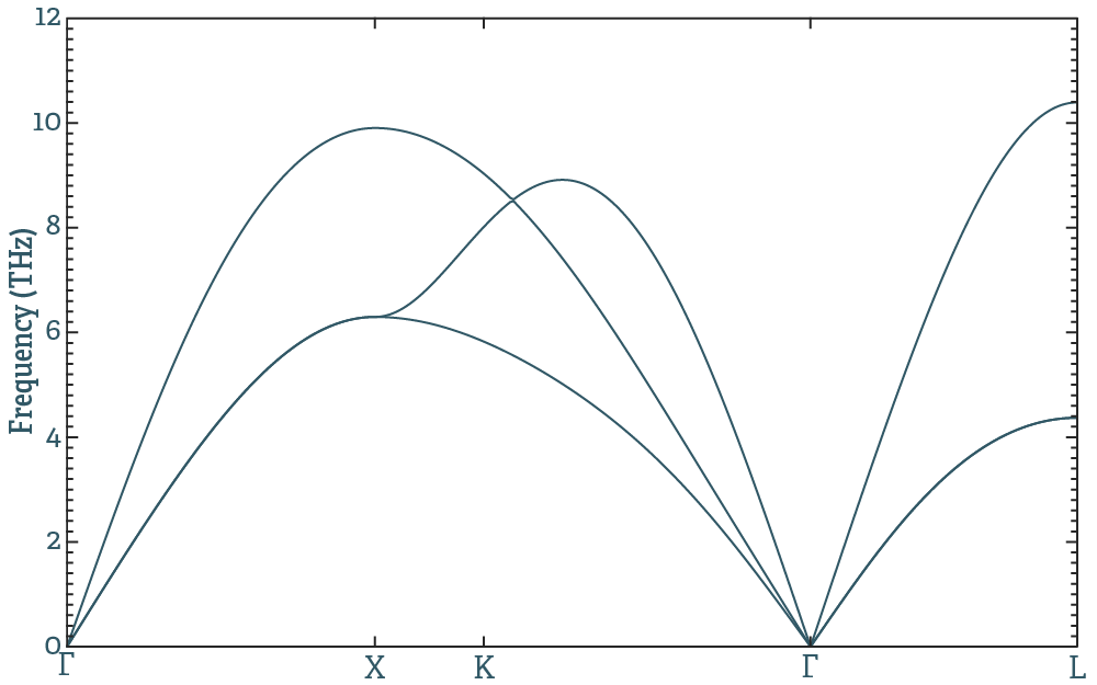
Frequency as a function of q-vector is written to outfile.dispersion_relations. If gnuplot is properly set up (if gnuplot just flashes, it's probably because it is missing the --persist option), you can run

gnuplot outfile.dispersion_relations.gnuplot

And you should see something like this:

If we want to know something about the broadening we need third order force constants. To get these, we rerun

extract_forceconstants -rc2 5 -rc3 3

And it will produce a new forceconstant file, outfile.forceconstant_thirdorder. Again, we need to copy (or link) it to an infile:

ln -s outfile.forceconstant_thirdorder infile.forceconstant_thirdorder

Once this is set up, we use the lineshape code to produce the phonon spectral function:

mpirun lineshape --path -qg 7 7 7 -ne 600 --temperature 800

and this produces, among other things, an outfile.sqe (and the hdf5 version of the same data, outfile.sqe.hdf5). I read this into matlab and plotted it with a logarithmic intensity scale, and the results look something like this:

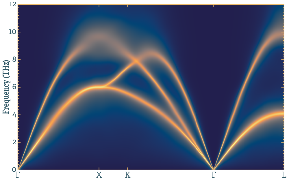
This is a sample matlab code snippet to produce this plot:

% read everything from file
fn=('outfile.sqe.hdf5');
x=h5read(fn,'/q_values');
y=h5read(fn,'/energy_values');
gz=h5read(fn,'/intensity');
xtck=h5read(fn,'/q_ticks');
xtcklabel=strsplit(h5readatt(fn,'/','q_tick_labels'));
energyunit=h5readatt(fn,'/','energy_unit');

% plot the results

figure(1); clf; hold on; box on;

[gy,gx]=meshgrid(y,x);
s=pcolor(gx,gy,log10(gz+1E-2));
set(s,'edgecolor','none','facecolor','interp')
set(gca,'xtick',xtck,'xticklabel',xtcklabel)
ylabel(['Energy (' energyunit ')'])
xlim([0 max(x)])
ylim([0 max(y)])

And an equivalent snippet using matplotlib

import matplotlib.pyplot as plt
import numpy as np
import h5py as h5
from matplotlib.colors import LogNorm

# open the sqe file
f = h5.File('outfile.sqe.hdf5','r')
# get axes and intensity
x = np.array(f.get('q_values'))
y = np.array(f.get('energy_values'))
gz = np.array(f.get('intensity'))
# add a little bit so that the logscale does not go nuts
gz=gz+1E-2
# for plotting, turn the axes into 2d arrays
gx, gy = np.meshgrid(x,y)
# x-ticks
xt = np.array(f.get('q_ticks'))
# labels for the x-ticks
xl = f.attrs.get('q_tick_labels').split()
# label for y-axis
yl = "Energy ("+f.attrs.get('energy_unit')+")"

plt.pcolormesh(gx, gy, gz, norm=LogNorm(vmin=gz.min(), vmax=gz.max()), cmap='viridis')
# set the limits of the plot to the limits of the data
plt.axis([x.min(), x.max(), y.min(), y.max()])
plt.xticks(xt,xl)
plt.ylabel(yl)

plt.show()

Read the documentation for the codes used, and familiarize yourself with their capabilities before moving on. A couple of things that should be very easy, and a final one that requires some thought:

• Change the q-point path through the Brillouin zone. First plot the dispersions along this new path, then the spectralfunction. hint.
• Plot the phonon DOS in units of meV from the second order force constants. Understand the difference between the different ways to integrate. hint.
• Get the broadened phonon DOS at some temperature. Try to understand the difference in integration technique when doing this, and the example above. hint.
• Get the phonon free energy at 450K. hint.
• Figure out what depends on what. If you have calculated the spectralfunction at 300K, and want to do it with a tighter q-point grid, from what step do you have to start over? If you want a longer cutoff for the second order force constants, from what step do you have to repeat the procedure?