Short description

Calculate phonon dispersions and related quantities. Per default, only the dispersions along a default path will be calculated. Options are available for calculating mode gruneisen parameters, phonon density of states projected in a variety of ways, thermodynamic quantities and pure data dumps.

Command line options:

Optional switches:

• --unit value, value in: thz,mev,icm
  default value thz
  Choose the output unit. The options are terahertz (in frequency, not angular frequency), inverse cm or meV.

• --nq_on_path value, -nq value
  default value 100
  Number of q-points between each high symmetry point

• --readpath, -rp
  default value .false.
  Read the q-point path from infile.qpoints_dispersion. Use crystal structure into to generate an example.

• --dos
  default value .false.
  Calculate the phonon DOS

• --qpoint_grid value#1 value#2 value#3, -qg value#1 value#2 value#3
  default value 26 26 26
  Density of q-point mesh for Brillouin zone integrations.

• --meshtype value, value in: 1,2,3
  default value 1
  Type of q-point mesh. 1 Is a Monkhorst-Pack mesh, 2 an FFT mesh and 3 my fancy wedge-based mesh with approximately the same density the grid-based meshes.

• --sigma value
  default value 1.0
  Global scaling factor for the Gaussian/adaptive Gaussian smearing. The default is determined procedurally, and scaled by this number.

• --readqmesh
  default value .false.
  Read the q-point mesh from file. To generate a q-mesh file, see the genkpoints utility.

• --integrationtype value, -it value, value in: 1,2,3,4
  default value 2
  Type of integration for the phonon DOS. 1 is Gaussian, 2 adaptive Gaussian and 3 Tetrahedron.

• --dospoints value
  default value 400
  Number of points on the frequency axis of the phonon dos.

• --temperature value
  default value -1
  Evaluate thermodynamic phonon properties at a single temperature.

• --temperature_range value#1 value#2 value#3
  default value -1 -1 -1
  Evaluate thermodynamic phonon properties for a series of temperatures, specify min, max and the number of points.

• --gruneisen
  default value .false.
  Use third order force constants to calculate mode Gruneisen parameters.

• --dumpgrid
  default value .false.
  Write files with q-vectors, frequencies, eigenvectors and group velocities for a grid.

• --help, -h
  Print this help message

• --version, -v
  Print version

Examples

phonon_dispersion_relations

phonon_dispersion_relations --dos -qgrid 24 24 24 -loto --integrationtype 2

This code calculates the phonon dispersions, $ \omega(\mathbf{q}) $. It can output dispersions along a line in the Brillouin zone, output frequencies on a grid, or calculate the phonon DOS. In addition it can calculate the mode Grüneisen parameters. By default, minimal input is needed, but many options to tailor the output exist.

Equations of motion in a harmonic crystal

As detailed in extract forceconstants we have mapped the Born-Oppenheimer to an effective potential. A model Hamiltonian truncated at the second order (a harmonic Hamiltonian) is given by¹

$$ \begin{equation} \hat H=\sum_{\kappa} \frac{\mathbf{p}_{\kappa}^2}{2m_{\kappa}} + \frac{1}{2} \sum_{\kappa\lambda}\sum_{\alpha\beta} \Phi_{\kappa\lambda}^{\alpha\beta} u^{\alpha}_{\kappa} u^{\beta}_{\lambda}\, \end{equation} $$

Where $\kappa,\lambda$ are indices to atoms, $\alpha,\beta$ Cartesian indices and $\mathbf{u}$ a displacement from equilibrium positions. To clarify, the instantaneous position of an atom is given by

$$ \begin{equation} \mathbf{r}_{\kappa} = \mathbf{R}_{\mu} + \boldsymbol{\tau}_{i} + \mathbf{u} \end{equation} $$

such that $\mathbf{R} +\boldsymbol{\tau}$ denote the equilibrium position of the atom. The lattice vector $\mathbf{R}$ locate the unit cell, $\boldsymbol{\tau}$ locate the atom in the unit cell, and $\mathbf{u}$ how far the atom has moved from the reference positions. Ignoring surface effects, we can write the equations of motion:

$$ \begin{equation} \ddot{\mathbf{u}}_{\mu i} m_{\mu i} = -\sum_{\nu j} \mathbf{\Phi}_{\mu i,\nu j}\mathbf{u}_{\nu j} \,. \end{equation} $$

Here we expanded the atom index $\kappa$ to the double index indicating cell $\mu$ and position $i$. Since we deal with infinite crystals with periodic boundary conditions, the equations of motion will not depend on cell index $\mu$, and that index can be dropped.

$$ \begin{equation}\label{eq:eqmotion1} \ddot{\mathbf{u}}_{i} m_{i} = -\sum_{\nu j} \mathbf{\Phi}_{\mu i,\nu j}\mathbf{u}_{\nu j}. \end{equation} $$

I prefer a truncated notation:

$$ \begin{equation} \ddot{\mathbf{u}}_{i} m_{i} = -\sum_{\mathbf{R}} \mathbf{\Phi}_{ij}\left( \mathbf{R} \right)\mathbf{u}_{j}. \end{equation} $$

Where $\mathbf{R}$ implies the cell index corresponding to atom $j$. To solve these equations of motion, we can use a plane-wave ansatz:

$$ \begin{equation} \mathbf{u}_{i}=\frac{1}{\sqrt{m_i}} \sum_{\mathbf{q}} A_{\mathbf{q}} \boldsymbol{\epsilon}_{\mathbf{q}}^{i} e^{ i \left(\mathbf{q} \cdot \mathbf{R} - \omega t \right) }. \end{equation} $$

Here the displacements are expressed as a sum of plane waves, or normal modes, each with wave vector $\mathbf{q}$ and frequency $\omega$. $\boldsymbol{\epsilon}$ is a polarisation vector, and $A_{\mathbf{q}}$ the normal mode amplitude. Substituting this into $\eqref{eq:eqmotion1}$ and exploiting the orthogonality of planes waves gives,

$$ \begin{split} \sqrt{m_i}\sum_{\mathbf{q}} \omega^2 A_{\mathbf{q}} \boldsymbol{\epsilon}_{\mathbf{q}}^{i} e^{ i \left(\mathbf{q} \cdot \mathbf{R}_i - \omega t \right) } = & \sum_{\mathbf{R}}\sum_{\mathbf{q}} \frac{A_{\mathbf{q}} \boldsymbol{\epsilon}_{\mathbf{q}}^{i}}{\sqrt{m_j}} \mathbf{\Phi}_{ij}\left( \mathbf{R}_j \right) e^{ i \left(\mathbf{q} \cdot \mathbf{R}_j - \omega t \right) } \\ % % \sum_{\mathbf{q}} \omega^2 A_{\mathbf{q}} \boldsymbol{\epsilon}_{\mathbf{q}}^{i} e^{ i \mathbf{q} \cdot \mathbf{R}_i } = & \sum_{\mathbf{R}}\sum_{\mathbf{q}} \frac{A_{\mathbf{q}} \boldsymbol{\epsilon}_{\mathbf{q}}^{i}}{\sqrt{m_i m_j}} \mathbf{\Phi}_{ij}\left( \mathbf{R}_j \right) e^{ i \mathbf{q} \cdot \mathbf{R}_j } \\ % % \sum_{\mathbf{q}'} \omega^2 A_{\mathbf{q}'} \boldsymbol{\epsilon}_{\mathbf{q}'}^{i} e^{ i \mathbf{q}' \cdot \mathbf{R}_i } e^{ -i \mathbf{q} \cdot \mathbf{R}_i } = & \sum_{\mathbf{R}}\sum_{\mathbf{q}'} \frac{A_{\mathbf{q}'} \boldsymbol{\epsilon}_{\mathbf{q}'}^{i}}{\sqrt{m_i m_j}} \mathbf{\Phi}_{ij}\left( \mathbf{R}_j \right) e^{ i \mathbf{q}' \cdot \mathbf{R}_j } e^{ -i \mathbf{q} \cdot \mathbf{R}_i } \\ % % \omega^2 A_{\mathbf{q}} \boldsymbol{\epsilon}_{\mathbf{q}}^{i} = & A_{\mathbf{q}} \boldsymbol{\epsilon}_{\mathbf{q}}^{i} \sum_{\mathbf{R}} \frac{\mathbf{\Phi}_{ij}\left( \mathbf{R}_j \right)}{\sqrt{m_i m_j}} e^{ i \mathbf{q} \cdot \mathbf{R}_j } \\ % % \omega^2_{\mathbf{q}} \boldsymbol{\epsilon}_{\mathbf{q}}= & \mathbf{\Phi}(\mathbf{q}) \boldsymbol{\epsilon}_{\mathbf{q}}\,, \end{split} $$

where the periodic boundary conditions limit the choices of $\mathbf{q}$ to a wave vector $\mathbf{q}$ in the first Brillouin zone. The dynamical matrix $\mathbf{\Phi}(\mathbf{q})$ is given by

$$ \begin{equation} \mathbf{\Phi}(\mathbf{q})= \begin{pmatrix} \mathbf{\Phi}_{11}(\mathbf{q}) & \cdots & \mathbf{\Phi}_{N 1}(\mathbf{q}) \\ \vdots & \ddots & \vdots \\ \mathbf{\Phi}_{1N}(\mathbf{q}) & \cdots & \mathbf{\Phi}_{N N}(\mathbf{q}) \\ \end{pmatrix} \end{equation} $$

This is the Fourier transform of the mass-weighted force constant matrix, where each $3 \times 3$ submatrix of the full $3N \times 3N$ is given by

$$ \begin{equation} \mathbf{\Phi}_{ij}(\mathbf{q})= \sum_{\mathbf{R}} \frac{ \mathbf{\Phi}_{ij}(\mathbf{R}) }{\sqrt{m_i m_j}} e^{i\mathbf{q}\cdot \mathbf{R}} \,. \end{equation} $$

The eigenvalues $\omega^2_{\mathbf{q}s}$ and eigenvectors $\boldsymbol{\epsilon}_{\mathbf{q}s}$ of the dynamical matrix denote the possible normal mode frequencies and polarizations of the system. The eigenvalues have the same periodicity as the reciprocal lattice; hence it is convenient to limit the solution to all vectors $\mathbf{q}$ in the first Brillouin zone. It is also worth defining the partial derivatives of the dynamical matrix:

$$ \begin{equation} \frac{\partial \mathbf{\Phi}_{ij}(\mathbf{q})}{\partial q_\alpha} = \sum_{\mathbf{R}} iR_\alpha \frac{ \mathbf{\Phi}_{ij}(\mathbf{R}) }{\sqrt{m_i m_j}} e^{i\mathbf{q}\cdot \mathbf{R}}. \end{equation} $$

By calculating the eigenvalues and eigenvectors of the dynamical matrix over the Brillouin zone, all thermodynamic quantities involving the atomic motions can be determined, as far as the harmonic approximation is valid. If you are curious where the amplitudes of the normal modes disappeared, see canonical configuration.

Long-ranged interactions in polar materials

When determining the dynamical matrix, the sum over lattice vectors $\mathbf{R}$ should in principle be carried out over all pairs. In practice, we assume that the interactions are zero beyond some cutoff (see extract forceconstants option -rc2), and truncate the sum. This is not a valid approach when dealing with polar material where the induced dipole-dipole interactions are essentially infinite-ranged. See for example Gonze & Lee.^{5 6} When dealing with these long-ranged electrostatics we start by defining the Born effective charge tensor:

$$ Z_{i}^{\alpha\beta} = \frac{\partial^2 U}{\partial \varepsilon^{\alpha} \partial u_{i}^{\beta}} $$

That is the mixed derivative of the energy with respect to electric field $\varepsilon$ and displacement $\mathbf{u}$. Displacing an atom from its equilibrium position induces a dipole, given by

$$ \mathbf{d}_{i} = \mathbf{Z}_{i}\mathbf{u}_{i} $$

The pairwise dipole-dipole interactions can be expressed as forceconstants:

$$ \begin{align} \Phi^{\textrm{dd}}|^{\alpha\beta}_{ij} & = \sum_{\gamma\delta} Z_{i}^{\alpha\gamma}Z_{j}^{\beta\delta} \widetilde{\Phi}^{\gamma\delta}_{ij} \\ \widetilde{\Phi}^{\alpha\beta}_{ij} & = \frac{1}{4\pi\epsilon_0} \frac{1}{\sqrt{\det \epsilon}} \left( \frac { \widetilde{\epsilon}^{\alpha\beta} } {|\Delta_{ij}|_{\epsilon}^{3}} -3 \frac {\Delta_{ij}^{\alpha}\Delta_{ij}^{\beta}} {|\Delta_{ij}|_{\epsilon}^{5}} \right) \end{align} $$

Here $\boldsymbol{\epsilon}$ is the dielectric tensor, $\widetilde{\boldsymbol{\epsilon}}=\boldsymbol{\epsilon}^{-1}$ its inverse and $\Delta$ realspace distances using the dielectric tensor as a metric:

$$ \begin{align} \mathbf{r}_{ij} & = \mathbf{R}_{j}+\mathbf{\tau}_j-\mathbf{\tau}_i \\ \mathbf{\Delta}_{ij} & =\widetilde{\boldsymbol{\epsilon}}\mathbf{r}_{ij} \\ |\Delta_{ij}|_{\epsilon} & = \sqrt{\mathbf{\Delta}_{ij} \cdot \mathbf{r}_{ij}} \end{align} $$

This poses an issue when calculating the dynamical matrix: the interactions die off as $~1/r^{3}$ which makes it necessary to extend the sum over lattice vectors to infinity. This is remedied with the usual Ewald technique:

$$ \widetilde{\mathbf{\Phi}}_{ij} (\mathbf{q})= \widetilde{\mathbf{\Phi}}^\textrm{r}+\widetilde{\mathbf{\Phi}}^\textrm{q}+\widetilde{\mathbf{\Phi}}^\textrm{c} $$

Dividing the sum into a realspace part, a reciprocal part and a connecting part. The realspace part is given by

$$ \begin{align} \widetilde{\mathbf{\Phi}}^\textrm{r}_{ij} & = -\frac{\Lambda^3}{4\pi\epsilon_0\sqrt{\det \epsilon}} \sum_{\mathbf{R}} \mathbf{H}(\Lambda \Delta_{ij},\Lambda|\Delta_{ij}|_{\epsilon}) e^{i \mathbf{q} \cdot \mathbf{R}} \\ %% \frac{\partial \widetilde{\mathbf{\Phi}}^\textrm{r}_{ij}}{\partial q_\alpha} & = -\frac{\Lambda^3}{4\pi\epsilon_0\sqrt{\det \epsilon}} \sum_{\mathbf{R}} iR_\alpha \mathbf{H}(\Lambda \Delta_{ij},\Lambda|\Delta_{ij}|_{\epsilon}) e^{i \mathbf{q} \cdot \mathbf{R}} \end{align} $$

where

$$ H_{\alpha\beta}(\mathbf{x},y) = \frac{x_{\alpha}x_{\beta} }{y^2} \left[ \frac{3\,\textrm{erfc}\,y}{y^3} + \frac{2 e^{-y^2}}{\sqrt{\pi}}\left(\frac{3}{y^2}+2 \right) \right] -\widetilde{\epsilon}_{\alpha\beta} \left[ \frac{\textrm{erfc}\,y}{y^3} + \frac{2 e^{-y}}{\sqrt{\pi} y^2 } \right]\,. $$

In reciprocal space we have

$$ \begin{align} % % Not derivative % \widetilde{\Phi}_\textrm{q}|_{ij} &= \sum_{\mathbf{K}=\mathbf{G}+\mathbf{q}} \chi_{ij}(\mathbf{K},\Lambda) \left( \mathbf{K}\otimes\mathbf{K} \right) \\ % % X-direction % \frac{\partial}{\partial q_x} \widetilde{\Phi}_\textrm{q}|_{ij} % &= \sum_{\mathbf{K}=\mathbf{G}+\mathbf{q}} \chi_{ij}(\mathbf{K},\Lambda) \left( \mathbf{K}\otimes\mathbf{K} \right) % \left( i\tau^x_{ij} - \left[\sum_{\alpha} K_\alpha \epsilon_{\alpha x} \right] \left[ \frac{1}{\|\mathbf{K}\|_{\epsilon}}+\frac{1}{4\Lambda^2} \right] \right) + % \chi_{ij}(\mathbf{K},\Lambda) \begin{pmatrix} 2K_x & K_y & K_z \\ K_y & 0 & 0 \\ K_z & 0 & 0 \end{pmatrix} \\ % % Y-direction % \frac{\partial}{\partial q_y} \widetilde{\Phi}_\textrm{q}|_{ij} % &= \sum_{\mathbf{K}=\mathbf{G}+\mathbf{q}} \chi_{ij}(\mathbf{K},\Lambda) \left( \mathbf{K}\otimes\mathbf{K} \right) % \left( i\tau^y_{ij} - \left[\sum_{\alpha} K_\alpha \epsilon_{\alpha y} \right] \left[ \frac{1}{\|\mathbf{K}\|_{\epsilon}}+\frac{1}{4\Lambda^2} \right] \right) + % \chi_{ij}(\mathbf{K},\Lambda) \begin{pmatrix} 0 & K_x & 0 \\ K_y & 2K_y & K_z \\ 0 & K_z & 0 \end{pmatrix}\\ % % Z-direction % \frac{\partial}{\partial q_z} \widetilde{\Phi}_\textrm{q}|_{ij} % &= \sum_{\mathbf{K}=\mathbf{G}+\mathbf{q}} \chi_{ij}(\mathbf{K},\Lambda) \left( \mathbf{K}\otimes\mathbf{K} \right) % \left( i\tau^z_{ij} - \left[\sum_{\alpha} K_\alpha \epsilon_{\alpha z} \right] \left[ \frac{1}{\|\mathbf{K}\|_{\epsilon}}+\frac{1}{4\Lambda^2} \right] \right) + % \chi_{ij}(\mathbf{K},\Lambda) \begin{pmatrix} 0 & 0 & K_x \\ 0 & 0 & K_y \\ K_z & K_y & 2K_z \end{pmatrix} \end{align} $$

where

$$ \begin{align} \chi_{ij}(\mathbf{K},\Lambda) & = \frac{1}{\Omega\epsilon_0} \frac{ \exp\left(i \mathbf{q} \cdot \mathbf{\tau}_{ij} \right) \exp\left( -\frac{\|\mathbf{K}\|_{\epsilon}}{4\Lambda^2} \right) } {\|\mathbf{K}\|_{\epsilon}} \\ %% \|\mathbf{K}\|_{\epsilon} & =\sum_{\alpha\beta}\epsilon_{\alpha\beta}K_\alpha K_\beta \end{align} $$

and finally a connecting part given by

$$ \widetilde{\mathbf{\Phi}}_\textrm{c}|_{ij}= \delta_{ij} \frac{\Lambda^3}{3 \epsilon_0 \pi^{3/2} \sqrt{ \det \boldsymbol{\epsilon} } } \widetilde{\boldsymbol{\epsilon}} $$

This expression is invariant for any $\Lambda>0$, which is chosen to make the real and reciprocal sums converge with as few terms as possible. Note that the Born charges are factored out from $\widetilde{\mathbf{\Phi}}$, and have to by multiplied in as described above. The derivatives with respect to $q$ are reproduced because they are useful when calculating the gradient of the dynamical matrix, needed when determining group velocities. In the long-wavelength limit, $\mathbf{q}\rightarrow 0$, the dipole-dipole dynamical matrix reduces to the familiar non-analytical term:

$$ \lim_{\mathbf{q}\rightarrow 0} \mathbf{\Phi}(\mathbf{q}) = \frac{1}{\Omega\epsilon_0} \frac{ \left(\mathbf{Z}_i\mathbf{q}\right) \otimes \left(\mathbf{Z}_j\mathbf{q}\right) }{\mathbf{q}^T\boldsymbol{\epsilon}\mathbf{q}} $$

This package implements three different ways of dealing with these long-ranged interactions. For historical reasons, the so-called mixed-space approach is available, but it should not be used except as an example of what not to do.

The technical issue is that the forces from a DFT calculation are not separated cleanly into "electrostatic longrange" and "everything else" components. The TDEP approach allows for two variants to separate this:

Separation approach 1

This is the approach proposed by Gonze & Lee⁶, only slightly adjusted since they assumed you start with reciprocal space dynamical matrices, whereas I start with realspace forceconstants. Algorithmically, it works like this:

• Define a $N_a \times N_b \times N_c$ suprecell, large enough that it snugly fits your realspace forceconstants.
• Calculate the electrostatic dynamical matrices on a $N_a \times N_b \times N_c$ $q$-mesh.
• Inverse fourier transform the electrostatic dynamical matrices to realspace forceconstants: $$ \mathbf{\Phi}^{\textrm{dd}}_{ij}(\mathbf{R}) =\frac{ \sqrt{m_i m_j} }{N_a N_b N_c} \sum_{\mathbf{q}} \Phi^{\textrm{dd}}_{ij}(\mathbf{q}) e^{-i\mathbf{q} \cdot \mathbf{R}} $$
• Subtract these from the realspace forceconstants: $$ \hat{\mathbf{\Phi}}_{ij}(\mathbf{R})= \mathbf{\Phi}_{ij}(\mathbf{R})- \mathbf{\Phi}^{\textrm{dd}}_{ij}(\mathbf{R}) $$
• Calculate the dynamical matrix as a sum of the short- and long-ranged contributions: $$ \mathbf{\Phi}_{ij}(\mathbf{q}) = \hat{\mathbf{\Phi}}_{ij}(\mathbf{R}) + \Phi^{\textrm{dd}}_{ij}(\mathbf{q}) $$

At $\mathbf{q}=0$ the non-analytcal contribution has to be added as well. This approach is reasonably robust, and works well in most materials. However, there are some aliasing contributions added since the realspace forceconstants are truncated by distance, and I propose a slight variation of this scheme:

Separation approach 2

This idea is similar in spirit, but does the separation into long- and short-ranged interactions at an earlier stage.

Mixed-space approach

This is implemented for historical reasons and for comparison, but disabled by default. It should not be used for anything, it is incorrect, and doing it right cost nothing.

Harmonic thermodynamics

In the previous section, we treated the vibrations of atoms classically, by solving Newton's equations of motion. Quantum-mechanically, vibrational normal modes can be represented as quasi-particles called phonons, quanta of thermal energy. We note that our normal mode transformation is a sum over eigenfunctions of independent harmonic oscillators. This allows us to write the position and momentum operators in terms of creation and annihilation operators (without loss of generality, we can contract the notation for phonon mode $s$ at wave vector $\mathbf{q}$ to a single index $\lambda$):

$$ \begin{align} \hat{u}_{i\alpha} = & \sqrt{ \frac{\hbar}{2N m_\alpha} } \sum_\lambda \frac{\epsilon_\lambda^{i\alpha}}{ \sqrt{ \omega_\lambda} } e^{i\mathbf{q}\cdot\mathbf{r}_i} \left( \hat{a}^{\mathstrut}_\lambda + \hat{a}^\dagger_\lambda \right) \\ % \hat{p}_{i\alpha} = & \sqrt{ \frac{\hbar m_\alpha}{2N} } \sum_\lambda \sqrt{ \omega_\lambda } \epsilon_\lambda^{i\alpha} e^{i\mathbf{q}\cdot\mathbf{r}_i-\pi/2} \left( \hat{a}^{\mathstrut}_\lambda - \hat{a}^\dagger_\lambda \right) % \end{align} $$

and their inverse

$$ \begin{align} \hat{a}^{\mathstrut}_{\lambda} = & \frac{1}{\sqrt{2N\hbar}} \sum_{i\alpha} \epsilon_\lambda^{i\alpha} e^{-i\mathbf{q}\cdot\mathbf{r}_i} \left( \sqrt{m_i \omega_\lambda} \hat{u}_{i\alpha}-i \frac{\hat{p}_{i\alpha}}{ \sqrt{ m_i \omega_\lambda }} \right) \\ % \hat{a}^\dagger_{\lambda} = & \frac{1}{\sqrt{2N\hbar}} \sum_{i\alpha} \epsilon_\lambda^{i\alpha} e^{i\mathbf{q}\cdot\mathbf{r}_i} \left( \sqrt{m_i \omega_\lambda} \hat{u}_{i\alpha}-i \frac{\hat{p}_{i\alpha}}{ \sqrt{ m_i \omega_\lambda }} \right) \end{align} $$

In terms of these operators, the vibrational Hamiltonian can be written as

$$ \begin{equation} \hat{H}=\sum_{\lambda}\hbar\omega_\lambda \left( \hat{a}^\dagger_\lambda \hat{a}^{\mathstrut}_\lambda + \frac{1}{2}\right)\,. \end{equation} $$

Since $\hat{a}^\dagger_\lambda \hat{a}^{\mathstrut}_\lambda$ are commutative operators, the Hamiltonian is that of a sum of uncoupled harmonic quantum oscillators, each having the partition function

$$ \begin{equation} Z_{\lambda}=\sum_{n=0}^{\infty}e^{-\beta (n +\frac{1}{2})\hbar\omega_{\lambda} } = \frac{ e^{-\beta \hbar\omega_{\lambda}/2 } }{1-e^{-\beta \hbar\omega_{\lambda}}} \end{equation} $$

that gives the total

$$ \begin{equation} Z=\prod_{\lambda} \frac{ e^{-\beta \hbar\omega_{\lambda}/2 } }{1-e^{-\beta \hbar\omega_{\lambda}}}. \end{equation} $$

From this we can get the Helmholtz (phonon) free energy:

$$ \begin{equation} F_{\textrm{ph}}= -k_B T \ln Z = \sum_{\lambda} \frac{\hbar \omega_{\lambda}}{2}+k_B T% \ln \left( 1- \exp \left( -\frac{\hbar \omega_{\lambda}}{k_B T} \right) \right) \end{equation} $$

In the conventional quasiharmonic approximation, the total free energy of the system (not considering any terms pertaining to magnetic or configurational degrees of freedom) can be expressed as

$$ \begin{equation} F = F_{\textrm{el}} + F_{\textrm{ph}}\,. \end{equation} $$

In the TDEP formalism it is not quite that simple.

Determining the free energy with TDEP

In the TDEP formalism,^4,3,2 with effective force constants, the phonon quasiparticles are different at each temperature. At fix temperature, they behave just like normal bosons, obeying Bose-Einstein statistics and so on. But changing the temperature will change both the occupation numbers and the states that are occupied. Moreover, in the harmonic approximation the baseline energy (with all atoms at their equilibrium positions) is that of the static lattice. With an effective Hamiltonian this baseline is a free parameter. The baseline shift is illustrated in the diagram below:

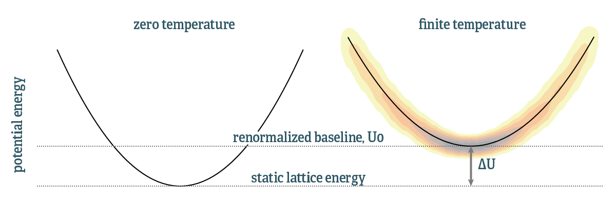
The density depicts the phase space samples used to fit the effective Hamiltonian. The reference energy, or baseline, has been shifted with respect to zero temperature. This baseline is determined by matching the potential energies of the samples of the Born-Oppenheimer surface, $U_{BO}$, and the potential energy of the TDEP model Hamiltonian:

$$ \begin{equation} \begin{split} \left\langle U_{\textrm{BO}} - U_{\textrm{TDEP}} \right\rangle & = \left\langle U_{\textrm{BO}} - U_0 -\frac{1}{2} \sum_{ij} \sum_{\alpha\beta} \Phi_{ij}^{\alpha\beta} u^{\alpha}_i u^{\beta}_j \right\rangle = 0 \\ U_0 & = \left\langle U_{\textrm{BO}} - \frac{1}{2} \sum_{ij} \sum_{\alpha\beta} \Phi_{ij}^{\alpha\beta} u^{\alpha}_i u^{\beta}_j \right\rangle \end{split} \end{equation} $$

Intuitively, this can be interpreted as that the TDEP force constants are determined by matching forces between the real and model system, in a similar manner we match the energies as well. The new baseline is conveniently expressed as a shift:

$$ \begin{equation} \Delta U = U_0-U_{\textrm{stat}} \end{equation} $$

Where $U_{\textrm{stat}}$ is the energy of the perfect lattice at 0K. The free energy is then (excluding configurational entropy, magnetic entropy etc.)

$$ \begin{equation} F = F_{\textrm{el}} + F_{\textrm{ph}} + \Delta U_0\,. \end{equation} $$

The entropy and heat capacity is not accessible from a single simulation. Since both the phonon free energy and baseline shift have non-trivial temperature dependencies, a series of calculations for different temperatures are needed, so that the entropy can be calculated via

$$ \begin{equation} S = -\left.\frac{dF}{dT}\right|_V \end{equation} $$

A series of calculations on a volume-temperature grid is required to calculate Gibbs free energy, with pressure explicitly calculated as

$$ \begin{equation} P = -\left.\frac{dF}{dV}\right|_T \end{equation} $$

Other dispersive properties

We determine group velocities via the Hellman-Feynmann theorem:

$$ \begin{equation} \nabla_{\mathbf{q}} \omega^2_s = \left\langle \epsilon_s(\mathbf{q}) \right| \nabla_{\mathbf{q}} \Phi(\mathbf{q}) \left| \epsilon_s(\mathbf{q}) \right\rangle \end{equation} $$

where the derivatives of the dynamical matrix are defined above, and

$$ \begin{equation} \mathbf{v}_{\mathbf{q}s} = \nabla_{\mathbf{q}} \omega_s(\mathbf{q})= \frac{1}{2\omega_s} \nabla_{\mathbf{q}} \omega_s^2(\mathbf{q}) \end{equation} $$

The only complications in using this expression is at wave vectors with degenerate frequencies, in those cases one has to average over the small group of the wave vector to obtain consistent group velocities.

The mode Grüneisen parameters are a measure of the sensitivity of the vibrational frequencies to volume changes. They are given by

$$ \begin{equation} \gamma_{\mathbf{q}s}=-\frac{V}{\omega_{\mathbf{q}s}}\frac{\partial \omega_{\mathbf{q}s}}{\partial V} \end{equation} $$

where $V$ is the volume and $\omega_{\mathbf{q}s}$ is the frequency of mode $s$ at wave vector $\mathbf{q}$. $\gamma_{\mathbf{q}s}$ can be obtained either by numerical differentiation of the phonon dispersion relations or from the third order force constants based on a perturbation approach:

$$ \begin{equation} \gamma_{\mathbf{q}s}=-\frac{1}{6\omega_{\mathbf{q}s}^2}\sum_{ijk\alpha\beta\gamma} \frac{\epsilon^{i\alpha\dagger}_{\mathbf{q}s} \epsilon^{j\beta}_{\mathbf{q}s}} {\sqrt{m_i m_j}} r_k^\gamma \Phi_{ijk}^{\alpha\beta\gamma}e^{i\mathbf{q}\cdot\ \mathbf{r}_j} \end{equation} $$

Here $\epsilon_{i\alpha}^{\mathbf{q}s}$ is component $\alpha$ associated eigenvector $\epsilon$ for atom $i$. $m_i$ is the mass of atom $i$, and $\mathbf{r}_i$ is the vector locating its position.

Density of states

Using --dos or --projected_dos_* will calculate the phonon density of states, given by

$$ g_s(\omega) = \frac{(2\pi)^3}{V} \int_{\mathrm{BZ}} \delta( \omega - \omega_{\mathbf{q}s}) d\mathbf{q} $$

per mode $s$, summing those up yields the total. The site projected density of states for site $i$ is given by

$$ g_i(\omega) = \frac{(2\pi)^3}{V} \sum_{s} \int_{\mathrm{BZ}} \left|\epsilon^i_{\mathbf{q}s}\right|^2 \delta( \omega - \omega_{\mathbf{q}s}) d\mathbf{q} $$

that, also sums to the total density of states.

Input files

• infile.ucposcar
• infile.forceconstant

Optional files:

• infile.qpoints_dispersion (to specify a path for the phonon dispersions)
• infile.lotosplitting (including the electrostatic corrections)
• infile.forceconstant_thirdorder (for the Grüneisen parameter)

Output files

Depending on options, the set of output files may differ. We start with the basic files that are written after running this code.

outfile.dispersion_relations

This file contains a list of $q$ points (in 1/Å) according to the chosen path (default or specified by the user in infile.qpoints_dispersions) and the frequencies per mode (in the specified units via --unit) for the corresponding points.

Row	Description
1	\( q_1 \qquad \omega_1 \qquad \omega_2 \qquad \ldots \qquad \omega_{3N_a} \)
2	\( q_2 \qquad \omega_1 \qquad \omega_2 \qquad \ldots \qquad \omega_{3N_a} \)
...	...

Not that the first column is for plotting purposes only. It serves to ensure that each line segment is scaled properly, since each segment contains a fix number of points.

outfile.group_velocities

This file contains the norm of the group velocities as a function of q. Format is identical to that of the dispersions:

Row	Description
1	\( q_1 \qquad |v_1| \qquad |v_2| \qquad \ldots \qquad |v_{3N_a}| \)
2	\( q_2 \qquad |v_1| \qquad |v_2| \qquad \ldots \qquad |v_{3N_a}| \)
...	...

The units are in km/s.

outfile.mode_gruneisen_parameters

In case you used --gruneisen, the mode Grüneisen parameters will be written, in a format similar to the dispersions and group velocities:

Row	Description
1	$ q_1 \qquad \gamma_1 \qquad \gamma_2 \qquad \ldots \qquad \gamma_{3N_a} $
2	$ q_2 \qquad \gamma_1 \qquad \gamma_2 \qquad \ldots \qquad \gamma_{3N_a} $
...	...

The units are in km/s.

outfile.phonon_dos

The first column is the list of frequencies and the second column in the density of states for this frequency, given in arbitrary units. Note that integrated density of states is normalized. One can calculate partial density of states (--projected_dos_mode); if the user specifies this option, an extra column will be added into the outfile.phonon_dos file for each type of atom. With --projected_dos_site the same thing happens but with an extra column for each atom in the unit cell.

Row	Description
1	$ \omega_1 \qquad g(\omega_1) \qquad g_1(\omega_1) \qquad \ldots \qquad g_{N}(\omega_1) $
2	$ \omega_2 \qquad g(\omega_2) \qquad g_1(\omega_2) \qquad \ldots \qquad g_{N}(\omega_2) $
...	...

The units are in states per energy unit, depending on choice of --unit. The total DOS normalizes to 3N independent of choice of unit.

outfile.free_energy

If one chooses the option --temperature_range or --temperature then this file will display a list of temperatures with corresponding temperatures, vibrational free energies, vibrational entropies and heat capacities.

Row	Description
1	$ T_1 \qquad F_{\textrm{vib}} \qquad S_{\textrm{vib}} \qquad C_v $
2	$ T_2 \qquad F_{\textrm{vib}} \qquad S_{\textrm{vib}} \qquad C_v $
...	...

Temperature is given in K, \( F_{\textrm{vib}} \) in eV/atom, \( S_\textrm{vib} \) in eV/K/atom and heat capacity in eV/K/atom.

outfile.mode_vibentropies

Using --modevib gives the mode-projected vibrational entropies:

Row	Description
1	\( T_1 \qquad S_{1} \qquad S_{2} \qquad \ldots \qquad S_{3N_a} \)
2	\( T_1 \qquad S_{1} \qquad S_{2} \qquad \ldots \qquad S_{3N_a} \)
...	...

Where all entropies are in eV/K/atom.

outfile.site_vibentropies

Using --sitevib gives the site-projected vibrational entropies:

Row	Description
1	\( T_1 \qquad S_{1} \qquad S_{2} \qquad \ldots \qquad S_{N_a} \)
2	\( T_1 \qquad S_{1} \qquad S_{2} \qquad \ldots \qquad S_{N_a} \)
...	...

The first column is the temperature, followed by one column per atom. All entropies are in eV/K/atom.

outfile.grid_dispersions.hdf5

Using option --dumpgrid writes all phonon properties for a grid in the BZ to an hdf5 file, that is self-documented.