atomic distribution
Short description
Calculates properties of the atomic distribution from molecular dynamics, such as mean square displacement, pair distribution function, vector distribution functions and probability densities. Useful for analysing simulations close to instabilities/phase transitions to have some idea where the atoms are.
Command line options:
Optional switches:
-
--cutoff value,-r value
default value 5.0
Consider pairs up to this distance, in A. -
--nbins value,-n value
default value 200
Number of bins in each dimension. -
--notransform
default value .false.
Do no rotate the coordinate systems of the vector distribution. By default, the coordinate system is aligned with the positive x-direction in the direction of the bond. -
--bintype value, value in:1,2,3
default value 1
Select the binning type for the vector distribution. 1 is straight binning (fastest), 2 is binning with a Gaussian, 3 is binning with a gaussian, but without the subpixel resolution. -
--stride value,-s value
default value 1
Use every N configuration instead of all. -
--help,-h
Print this help message -
--version,-v
Print version
Examples
atomic_distribution --cutoff 4.3
atomic_distribution --cutoff 4.3 --notransform
Long description
When using molecular dynamics, there are several ways to analyse the trajectories. This code implements a few of them. The TDEP method was originally meant to deal with dynamically unstable systems. It turns out the the most common problem for users was that the atoms did something during the simulation: what they thought was bcc Ti was no longer bcc Ti, but some halfway phase on it's way to transition to something.
So, before trying to get phonons and free energies and other things, it it useful to make sure that what is in your simulation box actually is what you think it is. A number of diagnostics is provided here.
Some background
The easiest measure is the mean square displacement:
$$ \textrm{msd}(t) = \frac{1}{N} \sum_i \left| \mathbf{r}_i(t)-\mathbf{r}_i(0) \right|^2 $$
where $\mathbf{r}_i(t)$ is the position of atom $i$ at time $t$. Having established that the system is at least still a solid we can look at the radial distribution function (or pair correlation function), defined as
$$ g(r) = \frac{ n(r) }{\rho 4 \pi r^2 dr} $$
where $\rho$ is the mean particle density, and $n(r)$ the number of particles in an infinitesimal shell of width $dr$. Usually, this is averaged over all atoms in the system. In this code, I project it onto symmetrically equivalent pairs, yielding a projected pair distribution:
$$ g_i(r) = {\rho 4 \pi r^2 dr} \sum_i \delta\left( \left|r_i\right|-r \right) $$
where the index $i$ corresponds to a coordination shell. The coordination shell is defined from the ideal lattice as set of pairs that can transform to each other via a spacegroup operation. Naturally, the sum over all projected PDFs yield the total.

Above is an example for ScF3. The peaks are well defined per pair, indicating that the system is still crystalline. In the projected picture, each coordination shell contributes one peak. Should on peak deviate strongly from a gaussian, it probably means that the system has undergone some internal shifts of the coordinates, altering the symmetry.
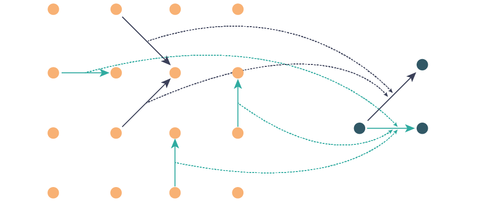
This code also calculates the vector distribution function, essentially three-dimensionsonal histograms of pair vectors. Schematically, it works like this: first I identify the symmetry inequivalent pair coordination shells (turqoise and blue arrows below). Each pair in the simulation cell gets a transformation associated with it (dashed lines) that takes them to the prototype vectors (connecting the dark blue atoms)
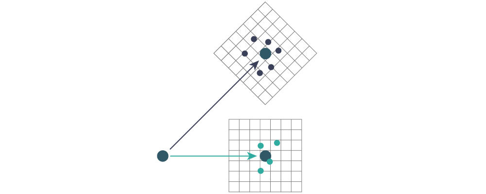
With these transformation rules, every pair from every timestep gets transformed, and binned in a histogram. The histogram is attached to the ideal bond, so that the origin coincides with the equilibrium pair vector. The coordinate system is also rotated such that the positive $z$-direction coincides with the pair vector, see the sketch below. The blue dots represent samples from pairs associated with blue vectors above, same for the green dots.
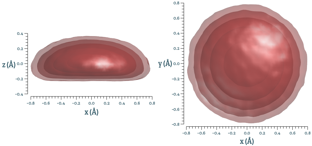
This results in three-dimensional distributions of pair vectors, one for each symmetry-distinct pair. This is a measure related to the pair correlation functions, but spatially resolved. If the distribution is given by $n(\mathbf{r})$, integrating this over spherical shells gives the pair correlation function described above. Using the same example as above, ScF3, isosurfaces of the distribution look like this for the nearest neighbour Sc-F pair:
Input files
Output files
outfile.mean_square_displacement.hdf5
The hdf file is self-explainatory. In addition, a plain-text outfile.mean_square_displacement is written with
| Row | Description |
|---|---|
| 1 | \( t_1 \qquad \textrm{msd}(t_1) \qquad \textrm{msd}_1(t_1) \qquad \ldots \qquad \textrm{msd}_{N_a}(t_1) \) |
| 2 | \( t_2 \qquad \textrm{msd}(t_2) \qquad \textrm{msd}_1(t_2) \qquad \ldots \qquad \textrm{msd}_{N_a}(t_2) \) |
| ... | ... |
Where the columns are time (in fs), mean square displacement (in Å2), followed by the partial mean square displacement per unique atom.
outfile.pair_distribution_function.hdf5
The hdf file is self-explainatory. Below is a matlab snippet that produces the plot above
clear all;
% filename
fn='outfile.pair_distribution_function.hdf5';
% number of unique atoms
na=h5readatt(fn,'/','number_unique_atoms');
% the total
x=h5read(fn,'/r_axis');
y=h5read(fn,'/radial_pair_distribution_function');
% the projected
for i=1:na
    xx{i}=h5read(fn,['/projected_r_axis_' num2str(i)]);
    yy{i}=h5read(fn,['/projected_pair_distribution_function_atom_' num2str(i)]);
end

figure(1); clf; hold on; box on;

% plot the total
plot(x,y)
% plot the projected
for i=1:na
for j=1:size(xx{i},1)
    plot(xx{i}(j,:),yy{i}(j,:))
end
end

set(gca,'xminortick','on','yminortick','on')
xlabel('Distance (A)')
ylabel('g(r)')
and an equivalent snippet using matplotlib:
import matplotlib.pyplot as plt
import numpy as np
import h5py as h5

# open the sqe file
f = h5.File('outfile.pair_distribution_function.hdf5','r')

# the total
x = np.array(f.get('r_axis'))
y = np.array(f.get('radial_pair_distribution_function'))
plt.plot(x,y)
# the projected
na = f.attrs.get('number_unique_atoms')
for i in range(na):
    x = np.array(f.get('projected_r_axis_'+str(i+1)))
    y = np.array(f.get('projected_pair_distribution_function_atom_'+str(i+1)))
    for j in range(x.shape[1]):
        plt.plot(x[:,j],y[:,j])

plt.xlabel("Distance (A)")
plt.ylabel("g(r)")
plt.show()
outfile.vector_distribution.hdf5
This file contains all the vector distribution histograms, the prototype vectors, the transformations to the correct coordinate systems and so on. The file is self-documented. The following is the matlab snippet used to create the plot above:
% file
fn='outfile.vector_distribution.hdf5';

% focus on one distribution, get the histogram
gv=h5read(fn,'/distribution_atom_1_shell_2');
% and the coordinates for the bin-centers
x=h5readatt(fn,'/distribution_atom_1_shell_2','bincenters');
% grids for plotting (always uniform)
[gx,gy,gz]=meshgrid(x,x,x);

figure(1); clf; hold on;

% number of isosurfaces
niv=6;
% values for the isosurfaces
iv=exp( linspace(log(0.01),log(1.5),niv) );

subplot(1,2,1); hold on;

    for i=1:niv
       p = patch(isosurface(gx,gy,gz,gv,iv(i)));
       isonormals(gx,gy,gz,gv, p)
       p.FaceColor = [0.7 0.1 0.1];
       p.EdgeColor = 'none';
       alpha(p,0.25);
    end

    daspect([1 1 1])
    view([0 1])
    camlight; lighting phong
    xlabel('x')
    ylabel('y')
    zlabel('z')

subplot(1,2,2); hold on;

for i=1:length(iv)
       p = patch(isosurface(gx,gy,gz,gv,iv(i)));
       isonormals(gx,gy,gz,gv, p)
       p.FaceColor = [0.7 0.1 0.1];
       p.EdgeColor = 'none';
       alpha(p,0.25);
    end

    daspect([1 1 1])
    view([0 0 1])
    camlight; lighting phong
    xlabel('x')
    ylabel('y')
    zlabel('z')
Note
I could not figure out an easy way to get decent-looking isosurfaces in matplotlib. Please tell me if you manage.